DIY alarm detection & phone notification system with Arduino Nano RP2040
GitHub repo
https://github.com/yoshidk6/alarm_detector_arduino
Intro
I recently bought a breadmaker (Panasonic SD-MDX4-K [Home Bakery Bistro] https://panasonic.jp/bakery/products/SD-MDX4.html) and while I absolutely love the bread, I frequently forget to take the bread off the machine as I cannot hear the beep coming from the kitchen.
So I decided to make my own beep sound detector with Arduino and send a notification to my phone! Arduino Nano RP2040 was a perfect fit as it has built-in mic and WiFi connectivity by default.
A couple of key elements in this project were:
- Use both the beep duration & audio frequency to only detect specific beep from my breadmaker
- Use Pushover service to send notifications (IFTTT often recommended, but phone notification became a premium feature)
Code breakdown
The project is divided into several key sections:
- WiFi Setup: Connect to the WiFi network.
- NTP Client: Synchronize the time using the Network Time Protocol (NTP).
- Audio Signal Processing: Capture and process audio signals to detect the beep sound.
- Pushover Notification: Send a notification when the beep is detected.
As described above, we combined two strategies to identify the beep sound: (1) look at specific frequency of sounds, and (2) look at the duration of the beep sounds. Combination of these resulted in almost no false-positive detections. Originally I looked for combining the duration of the sound & clock time from NTP, but looking at frequency turned out to be a better approach.
You can find section-by-section codes below with some explanations; see https://github.com/yoshidk6/alarm_detector_arduino for the full code.
WiFi Setup
First, we need to connect the Arduino to the WiFi network. The WiFiNINA library is used for this purpose. WiFi credentials are stored in a separate arduino_secrets.h file for security purposes.
arduino_secrets.h
#define SECRET_SSID "your_wifi_ssid"
#define SECRET_OPTIONAL_PASS "your_wifi_password"
#define SECRET_PUSHOVER_USER_KEY "your_pushover_user_key"
#define SECRET_PUSHOVER_API_KEY "your_pushover_api_key"
WiFi Setup Code
#include "arduino_secrets.h"
#include <WiFiNINA.h>

WiFiClient wifiClient;
char ssid[] = SECRET_SSID;
char pass[] = SECRET_OPTIONAL_PASS;
int status = WL_IDLE_STATUS;

void setup() {
  Serial.begin(9600);
  delay(1500);

  if (WiFi.status() == WL_NO_MODULE) {
    Serial.println("Communication with WiFi module failed!");
    while (true);
  }

  Serial.print("Attempting to connect to WPA SSID: ");
  Serial.println(ssid);
  WiFi.begin(ssid, pass);

  while (WiFi.status() != WL_CONNECTED) {}
}
NTP Client
We use the NTPClient library to synchronize the time. The time is updated every minutes (60000 milliseconds).
Here we are using GMT-8 (US Pacific Standard time) by specifying -28800, adjust this according to your timezone.
#include <WiFiUdp.h>
#include <NTPClient.h>

WiFiUDP ntpUDP;
NTPClient timeClient(ntpUDP, "pool.ntp.org", -28800, 60000); // GMT-8 (US Pacific Standard time)

void setup() {
  // Initialize WiFi and Serial (code from previous section)

  timeClient.begin();
  timeClient.update();
}
Audio Signal Processing
Frequency
The audio signals are captured using the built-in microphone on the Arduino Nano RP2040 Connect. We process the audio signals using FFT to determine the amplitude at a specific frequency (2050Hz in this case). The ApproxFFT.ino code from Instructables is used for FFT (Approx_FFT() function). The beep sound frequency of 2050Hz was separately determined by recording the beep sound and analyzing it using some free software in a local laptop (can’t remember the software name).
#include <PDM.h>

const int samples = 256; // Number of samples for the FFT
const int samplingFrequency = 14000; // Sampling frequency
short sampleBuffer[64];
short streamBuffer[samples]; // Sample stream buffer
int approxBuffer[samples];   // ApproxFFT sample buffer
volatile int samplesRead = 0;
volatile int sampleCount = 0;

int frequencyOfInterest = 2050; // Frequency to detect (2050Hz)
int amplitudeAtFrequency = 0;
int indexFreqSample = frequencyOfInterest * samples / samplingFrequency;

// Variables for max peak volume calculation
unsigned long startTime = 0;
const unsigned long extractionInterval = 5000000; // 5 seconds in microseconds
int maxAmplitudeDuringInterval = 0;

// Variables for alarm duration calculation
int amplitudeThreshold = 5000;
int volume_at_freq;

void setup() {
  // Initialize WiFi, Serial, and NTP (code from previous sections)

  PDM.onReceive(onPDMdata);
  PDM.setGain(20);
  if (!PDM.begin(1, samplingFrequency)) {
    Serial.println("Failed to start PDM!");
    while (1);
  }
}

void loop() {
  // Accumulate samples for FFT
  if (samplesRead) {
    for (int i = 0; i < samplesRead; i++) {
      streamBuffer[i + sampleCount] = sampleBuffer[i];
      approxBuffer[i + sampleCount] = sampleBuffer[i] / 2;
    }
    sampleCount += samplesRead;
    samplesRead = 0;
  }

  // Perform FFT when enough samples are accumulated
  if (sampleCount >= samples) {
    Approx_FFT(approxBuffer, samples, samplingFrequency);
    amplitudeAtFrequency = approxBuffer[indexFreqSample];

    sampleCount = 0;

    // Extract maximum amplitude
    if (amplitudeAtFrequency > maxAmplitudeDuringInterval) {
      maxAmplitudeDuringInterval = amplitudeAtFrequency;
    }

    // Check if 5 seconds have elapsed
    if (micros() - startTime >= extractionInterval) {
      Serial.print("Maximum amplitude during the last 5 seconds: ");
      Serial.println(maxAmplitudeDuringInterval);

      volume_at_freq = maxAmplitudeDuringInterval;

      maxAmplitudeDuringInterval = 0;
      startTime = micros();
    }

    // Process continuous signal
    processContSignal();
  }
}

void onPDMdata() {
  int bytesAvailable = PDM.available();
  PDM.read(sampleBuffer, bytesAvailable);
  samplesRead = bytesAvailable / 2;
}
Duration
Beep duration was also checked and found to have 7~8 total seconds. The continuous signals are analyzed as follows to detect the duration of the beep sound:
- isPrevSignalHigh: A flag to check the previous state of the signal.
- risePoint: The time when the signal goes HIGH.
- fallPoint: The time when the signal goes LOW.
- highTotalTime: The total duration time when the signal was HIGH.
- lowTime: The duration time when the signal was LOW.
The function checks if the amplitude is above the threshold and updates the variables accordingly. When the signal has been LOW for a sufficient duration, it calculates the total duration and checks if it meets specific criteria before sending a notification. This approach was coming from this blog post (written in Japanese)
// Process continuous signal duration
int limitTime = 1000000; // Silence time to determine the end of the sound (in microseconds)

int totalTime = 0;
int highTotalTime = 0;
int lowTime;
int firstRisePoint;
int risePoint;
int fallPoint;
bool isPrevSignalHigh = false;
int countSignalHigh = 0;

void processContSignal() {
  unsigned long currentTime = micros();

  // Check if the amplitude is above the threshold
  if (amplitudeAtFrequency > amplitudeThreshold) {
    if (!isPrevSignalHigh) {
      // Moment when the signal goes HIGH (rising edge)
      isPrevSignalHigh = true;
      risePoint = currentTime;
      countSignalHigh++;
      firstRisePoint = (countSignalHigh == 1) ? currentTime : firstRisePoint;
      Serial.println("Rising edge");
    }
  } else {
    if (isPrevSignalHigh) {
      // Moment when the signal goes LOW (falling edge)
      isPrevSignalHigh = false;
      fallPoint = currentTime;
      highTotalTime += currentTime - risePoint;
      Serial.print("Falling edge: current highTotalTime of ");
      Serial.print(highTotalTime / 1000);
      Serial.println(" ms");
    } else {
      lowTime = currentTime - fallPoint;

      // Check if the signal has been low for a sufficient duration
      if (countSignalHigh > 0 && lowTime > limitTime) {
        totalTime = currentTime - firstRisePoint - lowTime;
        Serial.println("End of alert:");
        Serial.print("current highTotalTime of ");
        Serial.print(highTotalTime / 1000);
        Serial.println(" ms");
        Serial.print("current totalTime of ");
        Serial.print(totalTime / 1000);
        Serial.println(" ms");

        // Check if the total time and high total time meet the criteria
        if (totalTime > 300000) {
          Serial.print(timeClient.getFormattedTime());
          Serial.print(" - ");
          Serial.print(totalTime / 1000);
          Serial.print("[");
          Serial.print(highTotalTime / 1000);
          Serial.println("]");

          // Check specific duration criteria before sending notification
          // if (totalTime > 500000) {
          //   sendNotification(); // Test code & learn the duration of alarm
          // }
          if (totalTime     > 7000000 && totalTime     < 8000000 &&
              highTotalTime > 2000000 && highTotalTime < 3000000) {
            sendNotification();
          }
        }

        // Reset variables for the next interval
        totalTime = 0;
        highTotalTime = 0;
        countSignalHigh = 0;
      }
    }
  }
}
Pushover Notification
When the beep sound is detected, a notification is sent to the Pushover account.
const char* pushoverAPI = "api.pushover.net";
const char* userKey = SECRET_PUSHOVER_USER_KEY;         // Pushover User Key
const char* apiToken = SECRET_PUSHOVER_API_KEY;       // Pushover API Token
const char* messageTitle = "Bread is ready!";

bool sendNotification() {
  Serial.println("Starting notification process...");

  // Attempt to connect to the Pushover API server with SSL
  if (!wifiClient.connectSSL("api.pushover.net", 443)) {
    Serial.println("Failed to connect to Pushover API server!");
    return false;
  }

  Serial.println("Connected to Pushover API server.");

  // Construct the HTTP POST payload
  String postData = "token=" + String(apiToken) +
                    "&user=" + String(userKey) +
                    "&title=" + String(messageTitle) +
                    "&message=" + String(timeClient.getFormattedTime()) +
                    "- Total time: " + String(totalTime) +
                    "- High total time: " + String(highTotalTime);


  // Construct and send the HTTP POST request
  wifiClient.println("POST /1/messages.json HTTP/1.1");
  wifiClient.println("Host: api.pushover.net");
  wifiClient.println("Connection: close");
  wifiClient.println("Content-Type: application/x-www-form-urlencoded");
  wifiClient.print("Content-Length: ");
  wifiClient.println(postData.length());
  wifiClient.println();
  wifiClient.print(postData);

  Serial.println("POST request sent. Waiting for response...");

  // Wait for the response from the server
  unsigned long timeout = millis();
  while (wifiClient.connected() && !wifiClient.available()) {
    if (millis() - timeout > 5000) { // 5-second timeout
      Serial.println("Timeout waiting for server response!");
      wifiClient.stop();
      return false;
    }
  }

  // Read the response from the server
  String response = "";
  while (wifiClient.available()) {
    response += wifiClient.readStringUntil('\n');
  }

  // Debugging: Print the response
  Serial.println("Response received:");
  Serial.println(response);

  // Close the connection
  wifiClient.stop();

  // Check for success in the response
  if (response.indexOf("\"status\":1") > -1) {
    Serial.println("Notification sent successfully!");
    return true;
  } else {
    Serial.println("Failed to send notification. Check the API response.");
    return false;
  }
}
References
- Example of detecting sounds and sending notifications: マイコン技術Navi: 【ESP32】特定の音が鳴ったらLINEで通知する(ご飯よ〜!を家族全員にお知らせシステム)
- FFT for analyzing beep sound: Instructables
- Get clock time: DigiKey
Docker上のnlmixrを使ってpopulation pharmacokinetics解析
2022.11.3追記
最近リリースされた nlmixr2 を使用すれば、Pythonをインストールすることなくpopulation pharmacokinetics解析を行うことができます。
Nonlinear Mixed Effects Models in Population PK/PD • nlmixr2
オープンソースの母集団薬物動態解析ソフトウェアであるnlmixr (https://ascpt.onlinelibrary.wiley.com/doi/full/10.1002/psp4.12445)を少し使ってみたのですが、Rとpythonを連携する必要があったりと立ち上げに少し手間取ったので、Dockerを使った環境設定について備忘録を残しておきます。
基本的には GitHub - yoshidk6/nlmixr.docker: docker for nlmixr に書いてある通りです。
目次
事前準備その1
まずはDockerのインストールが必要です。 Windowsの場合ここも結構面倒ですが、pythonとRの設定を色々いじるよりは楽かと思います。 特に手元にあるWindows環境がHome版だけだったので、Docker自体のインストールにも大分手間取りました。
以下のページを参考にし、まずはWSL2を導入します。 Windows 10 Home で WSL 2 + Docker を使う - Qiita
途中で確か
0x80070003か0x80370102のエラーがでて進めなくなったので、下を参考にBIOSの設定をいじったら無事WSL2を入れることができました。 Install WSL | Microsoft Learn
事前準備その2
ローカル環境内の作業用フォルダを用意します。
以下の例では C:\Users\USERID\Documents\test_nlmixr とします。
USERIDは自分のユーザー名で置き換えて下さい。
Docker imageを動かす
Docker Hub上にアップロードされているDockerイメージ (https://hub.docker.com/r/yoshidk6/nlmixr) を、以下のコマンドで起動します。
docker run -v C:/Users/USERID/Documents/test_nlmixr:/home/rstudio/docs -d -p 8787:8787 -e PASSWORD=nlmixr yoshidk6/nlmixr
ここでは-vオプションを使って、ローカル上のtest_nlmixrフォルダにDocker上からアクセス出来るように設定しています。
再び、USERIDは自分のユーザー名で置き換えて下さい。
下の様に、特にエラーなしで進めば成功しているはずです。

RStudio Serverに接続し、nlmixrを実行
localhost:8787 にブラウザから接続し、上で設定したパスワードを使ってログインします。
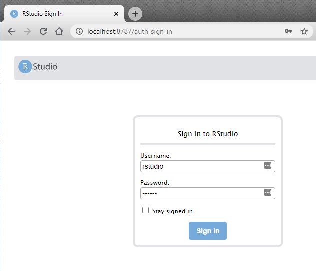
RStudioが無事起動したら、examplesフォルダ内にある example.R を開いて、コマンドを上から順に実行してみてください。29行目ではsaemによる推定結果が表示されるはずです。

また、44行目以降を実行すると、shinyMixRが起動し、GUI上でモデルファイルの操作などが出来ます。
Dockerの終了
本来はコマンドを使って操作すべきところですが、僕は怠惰なのでGUIに頼ってしまいます。
右下のメニュー内にあるクジラのアイコンを右クリックし、Dashboardを選ぶと、
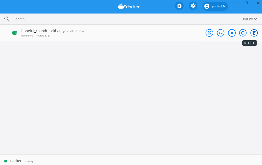
こんな感じで起動したコンテナを停止もしくは削除することが出来ます。
gretaパッケージをMac環境でインストールする
gretaパッケージは、TensorFlow Probabilityを活用してHamiltonian Monte Carlo法による統計モデリングを行うRのパッケージです。
StanやBUGSなどと違い、すべてR上でモデルの構築が出来るため、学習のハードルが低くなっているのが特徴です。
また、上のページにもある通り、モデルの構造を綺麗に表示してくれる機能が標準で備わっています。

TensorFlowを使っているためPythonをRにリンクする必要があり、Get started with greta • gretaに従っただけだとインストールがうまく行きませんでした。
デフォルトで選択されるPython環境をいじる必要があったので、備忘録的に手順を残しておきます。
"R reticulateの設定"などで検索するといろいろな情報が出てきますが、今回の手順は基本的に下のページに従いました。
PythonとTensorFlow, TensorFlow Probabilityをインストールする
r-tensorflowという名前のenvironmentをAnaconda上*1に作り、その中に適切なバージョンのPythonとTensorFlow, TensorFlow Probabilityをインストールするという流れになります。
- まずはAnacondaをインストールします Anaconda | Individual Edition
- Anacondaのプロンプト上(Macではターミナル)で以下のコマンドを打ちます
-
conda create -n r-tensorflow python=3.7 tensorflow=1.14 pyyaml requests Pillow pip numpy=1.16 -
conda activate r-tensorflow -
pip install tensorflow-probability==0.7
-
Rに結びつけるPythonのバージョン設定
Rにreticulateをインストールし、Pythonの環境を設定します。
Mac上(MacOS 10.14 Mojave)だとデフォルトではPython 2.xが選ばれてしまい、毎回Rを起動するたびにPythonの環境を選ぶ必要があって面倒です。
そのため、デフォルトで使うPythonを~/.Rprofileで設定してしまいます。
グローバルに設定を変えたくない場合は、プロジェクトごとに設定することも出来るはずです。
- reticulateをインストールする
install.packages("reticulate") - RStudio上で.Rprofileを開く
file.edit(file.path("~", ".Rprofile")) - 次のコマンドを.Rprofileに追記して保存する
reticulate::use_condaenv("r-tensorflow") - Rを再起動し、
reticulate::py_config()を打って r-tensorflow が選ばれていることを確認します
gretaのインストール
R/RStudio上でgretaをインストールします。
install.packages("greta")library(greta)
動作確認
ここまでの手順がエラーなく進めば、gretaが使えるようになっているはずです。
Get started with greta • greta上にある簡単な例を試してみてください。
library(greta)

# data
x <- as_data(iris$Petal.Length)
y <- as_data(iris$Sepal.Length)

# variables and priors
int <- normal(0, 1)
coef <- normal(0, 3)
sd <- student(3, 0, 1, truncation = c(0, Inf))

# operations
mean <- int + coef * x

# likelihood
distribution(y) <- normal(mean, sd)

# defining the model
m <- model(int, coef, sd)

# plotting
# plot(m) # This works only if you installed igraph and DiagrammeR

# sampling
draws <- mcmc(m, n_samples = 1000)

# result summary
summary(draws)
*1:Anaconda上のPython/TensorFlowだとサンプリング速度が2-8倍になるそうです。
Simulating parametric survival model with parametric bootstrap to capture uncertainty
I recently released an R package on CRAN calledsurvParamSim for parametric survival simulation, and here want to describe a bit more on details & motivations behind developing this package.
Parametric Survival Simulation with Parameter Uncertainty • survParamSim
The purpose of survParamSim is to package the R functions developed by a great scientist, the late Laurent Claret, and streamline the function definition/APIs to make these widely available to the public.
Laurent developed these functions for his pioneering works in applying tumor growth inhibition models for clinical outcome predictions of oncology studies, such as the one below.
clincancerres.aacrjournals.org
Explaining the theory behind his works is well beyond the scope of this short blog post, but the key technical highlight is that we are using parametric survival models with various covariates for predicting survival profiles and treatment benefits. In applying these workflows in the context of drug development (or maybe in most of other contexts), we want to make a prediction of not only the mean survival profiles but also the uncertainties associated with model predictions.
There are mainly two sources of uncertainty for such survival predictions. The first one is due to the nature of the survival prediction: because survival (or rather failure) is modeled as probabilistic processes, a predicted survival curve for a group will never be identical after multiple simulations. There is another source of uncertainty, which is the uncertainty associated with model parameters, such as coefficients associated with covariates in the model.
The first element is fairly straightforward to evaluate - we can run simulations many times and quantify how variable the survival curves can be by looking at prediction intervals. For example, we expect the prediction interval to generally get narrower if we make a prediction with larger number of patients. However, for the second part, there is not a readily available method for exploration to my (limited) knowledge. survival::predict.survreg() has se.fit option, but it is not straightforward to carry the output from this option for making predicted survival profiles of a group.
These are the main reasons for putting together this package - to enable the incorporation of above two sources of uncertainty in survival predictions, using parametric models obtained with survival::survreg(). For the second element of the uncertainty, we are using parametric bootstrap from variance-covariance matrix of the model parameter estimates.
Example
The code below is essentially the same as the one on GitHub pages, just showing a simple work flow to give you a sense of what to expect in terms of outputs. Vignette here has a bit more explanations on the workflow.
For this example, we use colon dataset in survival package, where the treatment benefit of Levamisole+5-FU was compared with control (called as Obs). Various covariates were further explored, such as extent of tumor local spread.
First, you would run survreg to fit parametric survival model:
library(tidyverse)
library(survival)
library(survParamSim)

set.seed(12345)

# ref for dataset https://vincentarelbundock.github.io/Rdatasets/doc/survival/colon.html
colon2 <-
  as_tibble(colon) %>%
  # recurrence only and not including Lev alone arm
  filter(rx != "Lev", etype == 1) %>%
  # Same definition as Lin et al, 1994
  mutate(rx = factor(rx, levels = c("Obs", "Lev+5FU")),
         depth = as.numeric(extent <= 2))
Here we have two covariates, node4 and depth, in addition to the treatment assignment rx.
fit.colon <- survreg(Surv(time, status) ~ rx + node4 + depth,
                     data = colon2, dist = "lognormal")
Next, parametric bootstrap simulation can be run with surv_param_sim() function from this package:
sim <-
  surv_param_sim(object = fit.colon, newdata = colon2,
                 censor.dur = c(1800, 3000),
                 # Simulating only 100 times to make the example go fast
                 n.rep = 100)
The output object merely has raw simulated survival data with 100 repetition (defined by n.rep argument).
You can find what options you have on this output by simply printing the object.
sim
#> ---- Simulated survival data with the following model ----
#> survreg(formula = Surv(time, status) ~ rx + node4 + depth, data = colon2,
#>     dist = "lognormal")
#>
#> * Use `extract_sim()` function to extract individual simulated survivals
#> * Use `calc_km_pi()` function to get survival curves and median survival time
#> * Use `calc_hr_pi()` function to get hazard ratio
#>
#> * Settings:
#>     #simulations: 100
#>     #subjects: 619 (without NA in model variables)
To visualize simulated survival curves with uncertainly, you can use calc_km_pi() and plot_km_pi() functions sequentially.
You can also specify faceting/grouping with trt and group input arguments.
km.pi <- calc_km_pi(sim, trt = "rx", group = c("node4", "depth"))

km.pi
#> ---- Simulated and observed (if calculated) survival curves ----
#> * Use `extract_median_surv()` to extract median survival times
#> * Use `extract_km_pi()` to extract prediction intervals of K-M curves
#> * Use `plot_km_pi()` to draw survival curves
#>
#> * Settings:
#>     trt: rx
#>     group: node4
#>     pi.range: 0.95
#>     calc.obs: TRUE

plot_km_pi(km.pi) +
  theme(legend.position = "bottom") +
  labs(y = "Recurrence free rate") +
  expand_limits(y = 0)

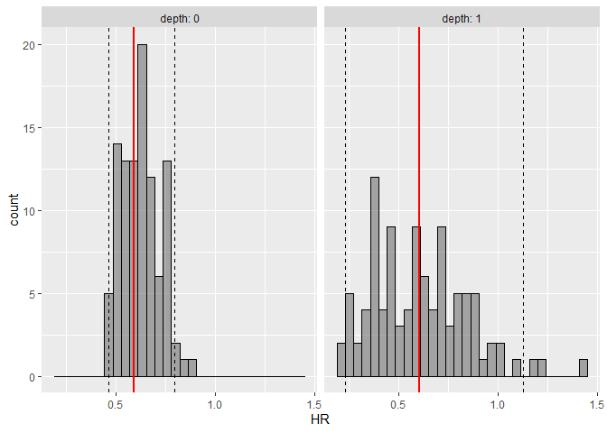
Similarly, you can visualize hazard ratios and prediction intervals with calc_hr_pi() and plot_hr_pi() functions.
hr.pi <- calc_hr_pi(sim, trt = "rx", group = c("depth"))

hr.pi
#> ---- Simulated and observed (if calculated) hazard ratio ----
#> * Use `extract_hr_pi()` to extract prediction intervals and observed HR
#> * Use `extract_hr()` to extract individual simulated HRs
#> * Use `plot_hr_pi()` to draw histogram of predicted HR
#>
#> * Settings:
#>     trt: rx
#>          (Lev+5FU as test trt, Obs as control)
#>     group: depth
#>     pi.range: 0.95
#>     calc.obs: TRUE
plot_hr_pi(hr.pi)
rstanやrstanarm等をWindows上でソースからインストールする時の設定
最近これに従って(Step by step guide for creating a package that depends on RStan • rstantools)RStanを使用するRのパッケージを作っていたのですが、どうもdevtools::install()やdevtools::build(binary = TRUE)などコンパイルを要するステップに入るとエラーが出てインストール出来ないという状況に陥りました。
いろいろ調べると、どうやらカスタムパッケージの問題ではなく、コンパイルの設定自体に問題があり、RStanやRStanArmもソースからインストール出来ないことが分かったので、対処法をメモしておきたいと思います。
ちなみに、コンピューターはWindows 7 or 10を使っているので、もしかしたらMac等では問題なく進むのかもしれません。
RStanのWikiに書かれているステップを実行する
まずは下の2つのページに書かれているステップに従い、(1) C++ Toolchainのインストールと(2) Makevarsファイルの設定(2つ目のページの Configuration 項)を行います。
- RStan Getting Started · stan-dev/rstan Wiki · GitHub
- Installing RStan from source on Windows · stan-dev/rstan Wiki · GitHub
g++のバージョンを確認する
通常は問題ないはずですが、僕の環境では他のプログラム用の古いバージョンのg++がPATH上で優先されてしまっていて、コンパイル時にエラーを起こしてしまっていました。
R上で以下のコードを打ち、バージョンが4.9以降だったら問題ありません。
system("g++ -v")
もしそうでない場合には、環境変数のPATHの頭に以下を追記します。
C:\Rtools\bin;C:\Rtools\mingw_64\bin;C:\Rtools\mingw_32\bin;
Makevar.winと.Rprofileを編集する
本当は最初のステップだけで上手く行くはずなのですが、僕の環境では上の手順を辿っても上手くいきませんでした。 *1 これを回避するために、Makevars.winと.Rprofileを編集する必要がありました。
Makevars.win
Makevars.winの位置はfile.path(Sys.getenv("HOME"), ".R")で、Windowsだと通常は C:/Users/USERNAME/Documents/.R/内にあります。
Makevars.win内の二行目のこれを
CXX14 = g++ -m$(WIN) -std=c++1y
以下のものに変更します。
CXX14 = $(BINPREF)g++ -m$(WIN) -std=c++1y
.Rprofile
.RprofileはSys.getenv("HOME")にあるはずですが、無ければ作成してください。上と同様に、Windowsだと通常は C:/Users/USERNAME/Documents/内に置かれます。
このファイル内に以下の行を追加してください。
Sys.setenv(BINPREF = "C:/RTools/mingw_$(WIN)/bin/")
*1:見たところ32ビット版のバイナリを作る時に64ビット版のg++を使ってしまっているようなので、PATH周りの問題かもしれません。
Using purrr's map family functions in dplyr::mutate
map family functions of the purrr package are very useful for using non-vectorized functions in dplyr::mutate chain (see GitHub - jennybc/row-oriented-workflows: Row-oriented workflows in R with the tidyverse or https://www.jimhester.com/2018/04/12/vectorize/).
I encounter the needs for this especially when dealing with nested data frames.
One of the drawbacks is that name/input argument assignments become confusing when you want to use more than two columns of your data frames (and using pmap family) for the function of interest.
This post first briefly review how mutate works in combination with map or map2, then provide two approaches to avoid confusions around name assignments when using pmap.
- How mutate works with vectorized functions
- Non-vectorized function with one or two input arguments (map or map2)
- Non-vectorized function with three or more input arguments (pmap)
How mutate works with vectorized functions
In most cases, the processes you want to do in mutate is vectorized and there is no need to use map family function.
This works because the output from the function of interest (c in the example below) has the same length as the original data frame, and mutate only need to append one column to the data frame.
library(tidyverse)

df0 <- tibble(a = 1:3, b = 4:6)

df0 %>% mutate(c = a + b)
Non-vectorized function with one or two input arguments (map or map2)
Imagine that we want to create a new column containing arithmetic progressions in each row [ref (in Japanese)].
Since seq function is not vectorized, we cannot directly use this in mutate chain.
df1 <- tibble(a = c(1, 2), b = c(3, 6), c = c(8, 10))

df1 %>% mutate(d = seq(a, b))
# Error in mutate_impl(.data, dots) : Evaluation error: 'from' must be of length 1.
Instead, we can use map family function here.
map family function take list(s) as input arguments and apply the function of interest using each element of the given lists.
Because each column of data frames in R is a list, map works very well in combination.
In this example, we want to provide two input arguments to the seq function, from and to.
map2 is the appropriate function for this.
df2 <- df1 %>% mutate(d = map2(a, b, seq))

as.data.frame(df2)
#  a b  c             d
#1 1 3  8       1, 2, 3
#2 2 6 10 2, 3, 4, 5, 6
The figure below shows how map function handles this process in mutate chain.
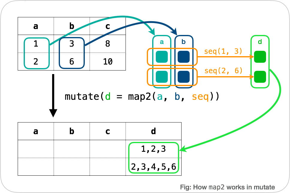
Like you do with map function outside mutate, we can use map_dbl or map_chr to create columns with double or character types.
If we want to explicitly specify names of the argument, .x and .y can be used.
See what happens with this:
df2 <- mutate(df1, d = map2(a, b, ~seq(.y, .x)))

as.data.frame(df2)
Non-vectorized function with three or more input arguments (pmap)
Assignment of column names become confusing when using three or more columns, because we don't have shorthand like .x or .y any more.
Let's take a look at the following example using rnorm function.
Case example
Generate a list of random numbers for each row with
rnormfunction. Each row of the original data frame contain different value ofmean,sd,n.
We will first prepare a data frame with columns corresponding to mean, sd, n, and apply rnorm function for each row using pmap.
Each element of the new column data contains a vector of random samples *1.
This type of structure is called as "nested data frames" and there are many resources on this, such as 25 Many models | R for Data Science.
A simple case
If your data frame has the exact same names and numbers of columns to the input arguments of the function of interest, a simple syntax like the one below works *2.
df4 <-
  tribble(~mean, ~sd, ~n,
          1,  0.03, 2,
          10, 0.1,  4,
          5,  0.1,  4)

df4.2 <-
  df4 %>%
  mutate(data = pmap(., rnorm))

as.data.frame(df4.2)
One caution is that the syntax like the one below doesn't work.
pmap thinks that you are calling rnorm(df4$n, df4$mean, df4$sd) for each row, and each element of the new column contain three random samples from the same list of mean and sd.
*3
df4 %>% mutate(data = pmap(., ~rnorm(n, mean, sd))) %>% as.data.frame() # Wrong answer
Number of columns > Number of input arguments
In most cases, however, you will have more columns than the input arguments.
pmap complains in this case, saying that you have unused argument.
df5 <-
  tribble(~mean, ~sd, ~dummy, ~n,
          1,  0.03, "a", 2,
          10, 0.1,  "b", 4,
          5,  0.1,  "c", 4)

df5 %>% mutate(data = pmap(., rnorm))  # Error
There are two ways to avoid this error.
Make a small list on the fly
The first method is to create a small list that only contains the necessary columns (Ref: Dplyr: Alternatives to rowwise - tidyverse - RStudio Community )
df5.2 <-
  df5 %>%
  mutate(data = pmap(list(n=n, mean=mean, sd=sd), rnorm))

as.data.frame(df5.2)
Here, list(n=n, mean=mean, sd=sd) create a new list with three vectors named n, mean, and sd, which serves the same purpose as the df4 data frame in the above example.
Mind that if you don't give names to the elements of the new list, the order of the list items will be used to associate with input arguments of rnorm.
My recommendation is to always assign names to the list elements.
df5 %>% mutate(data = pmap(list(n, mean, sd), rnorm)) # Correct but not recommended
df5 %>% mutate(data = pmap(list(mean, sd, n), rnorm)) # Wrong answer
Use ... to ignore unused columns
The second method is to absorb unused columns with ... (Ref: Map over multiple inputs simultaneously. — map2 • purrr).
A syntax like the one below works because pmap automatically associate names of the input list and names in function().
In other word, columns names of the data frame must match the variable names in the function().
df5.3 <-
  df5 %>%
  mutate(data = pmap(., function(n, mean, sd, ...) rnorm(n=n, mean=mean, sd=sd)))

as.data.frame(df5.3)
Input arguments of function() and rnorm() are not automatically associated with names. It is recommended to explicitly associate input argument name for the function of interest (rnorm in this case).
df5 %>% mutate(data = pmap(., function(n, mean, sd, ...) rnorm(n, mean, sd))) # Correct but not recommended
df5 %>% mutate(data = pmap(., function(n, mean, sd, ...) rnorm(mean, sd, n))) # Wrong answer
df5 %>% mutate(data = pmap(., function(mean, sd, n, ...) rnorm(mean, sd, n))) # Wrong answer
A syntax like the one below gives unexpected outputs, as you saw in the df4 example.
df5 %>% mutate(data = pmap(., function(...) rnorm(n=n, mean=mean, sd=sd))) # Wrong answer
Column names are different from the input argument names
You can use either of the two approaches above.
df6 <-
  tribble(~mean1, ~sd1, ~dummy, ~n1,
          1,  0.03, "a", 2,
          10, 0.1,  "b", 4,
          5,  0.1,  "c", 4)

df6.2 <-
  df6 %>% mutate(data = pmap(list(mean=mean1, sd=sd1, n=n1), rnorm))
as.data.frame(df6.2)

df6.3 <-
  df6 %>% mutate(data = pmap(., function(n1, mean1, sd1, ...) rnorm(n=n1, mean=mean1, sd=sd1)))
as.data.frame(df6.3)
*1:In the examples below (and above), we further use as.data.frame function to exposure actual numbers of vectors
*2:This works even if the order of the columns is different from the order of input arguments
*3:This happens because rnorm is actually vectorized. See ?rnorm: If length(n) > 1, the length is taken to be the number required.
dplyr::mutate内でベクトル化されていない関数を使う - purrr::pmapでのカラム名の対応付け
Rのデータフレームの各行に対して処理を行いたいが、関数をベクトル化することが難しい場合*1には、下で簡単に書くようにmutateとmapを組み合わせると非常に便利です。しかし、map内で定義する関数の入力値が3つ以上になると話が少しややこしくなります。納得するまで結構混乱したので、自分の備忘録も兼ねて記事にしておくことにしました。
通常のmutateを使った処理
殆どの場合、mutate内で行う処理(例えば+、*、ifelse等)はベクトル化されているので、出力値(下のケースではc)が他の列と同じ長さになり、元のデータフレームに追加されます。
library(tidyverse)

df0 <- tibble(a = 1:3, b = 4:6)

df0 %>% mutate(c = a + b)
各行について別々に処理、入力値が2つまでの場合
こちらにあるように、データフレームの各行に対して等差数列を作成する例を考えてみます。
このとき、seq関数はベクトル化されていないため、以下のように書くとエラーになります。
df1 <- tibble(a = c(1, 2), b = c(3, 6), c = c(8, 10))

df %>% mutate(d = seq(x, y))
# Error in mutate_impl(.data, dots) : Evaluation error: 'from' must be of length 1.
ここでmap系関数の出番です。
map系関数は、リストを引数とし、リスト内の各要素に対して与えられた関数を適用した結果を返すという働きを持っています。
Rのデータフレームは各列がそれぞれリストとなっているので、map系巻数と相性が良くなっています。
今回の例ではseq関数にfromとtoの2つの引数を与えたいので、map2関数を使います。
df2 <- df1 %>% mutate(d = map2(a, b, seq))

print(df2$d)
下にこの処理がどのように行われているかのイメージ図を貼ってみました。
もちろん、使用したい処理が一つの引数のみを取る場合はmapを使えばいいですし、作成する列をdoubleやcharacter型にしたければmap_dblやmap_chrなどを使います。
また、mapやmap2では、関数内で明示的に引数を指定したい場合、.xや.yを使います。例えば、上の例でdf2 <- mutate(df1, d = map2(a, b, ~seq(.y, .x)))を実行してみてください。
各行について別々に処理、入力値が3つ以上の場合
この様にmap系関数を使うと、ベクトル化されていない処理をmutate内で簡潔に書くことが出来ます。
3つ以上のカラムを使用したい場合、同様にpmapを使うことになるのですが、カラム名と関数の引数名の対応付けが少し複雑になります。
以下の例を用いて、どのように対応付けを行うことができるのか見ていきます。
使用する例
複数の平均値・標準偏差の組み合わせについて、それぞれ異なった数の乱数を
rnorm関数を用いて算出したい。
ここではまず、mean、sd、nに対応する3つのカラムを持ったデータフレームを作成し、各行ごとにrnorm関数を適用して乱数を発生させています。新しく生成されたカラムdataには、各行ごとに乱数値を保持したベクトルが格納されます。
結果を見やすくするため、この例では更にunnnest()関数を用いて縦長のデータフレームに変換していますが、変換せずにそのままmap系関数を使って処理を続けていくことも可能です。
ネスト化周りに関してはR4DSなど色々と解説があると思うので、馴染みのない方はそちらも参考にしてみてください。
- R for Data Science
- Rではじめるデータサイエンス、 20.2.1 入れ子データ
- tidyverse脳になって階層構造のあるデータフレームを使いこなそう
単純な例
データフレーム内のカラムが、pmap内で使用する関数の引数と個数・名前共に一致する場合にのみ、以下のような簡潔な文法が通じます。
df4 <-
  tribble(~mean, ~sd, ~n,
          1,  0.03, 2,
          10, 0.1,  4,
          5,  0.1,  4)

df4 %>% mutate(data = pmap(., rnorm)) %>% unnest()
ちなみに、下のような書き方だと、rnorm内の入力はdf4$n df4$mean df4$sdであると見做されてしまい、想定していない結果となってしまいます。
df4 %>% mutate(data = pmap(., ~rnorm(n, mean, sd))) %>% unnest() # Wrong answer
余分なカラムが含まれている場合
実際には、カラム数が関数の引数の数と一致するという状況は非常に稀だと思います。 余計なカラムが含まれていると、unused argumentがあると言って怒られます。
df5 <-
  tribble(~mean, ~sd, ~dummy, ~n,
          1,  0.03, "a", 2,
          10, 0.1,  "b", 4,
          5,  0.1,  "c", 4)

df5 %>% mutate(data = pmap(., rnorm))  # Error
これを回避するには、2つの方法があります。
小さいリストを作ってしまう
1つ目は、pmapの第一引数をdf4のようなリストにその場で変えてしまう方法です。(参照: Dplyr: Alternatives to rowwise - tidyverse - RStudio Community )
df5 %>% mutate(data = pmap(list(n=n, mean=mean, sd=sd), rnorm)) %>% unnest()
注意点として、下のようにリスト内要素に名前をつけないと、rnormへの受け渡しが順序のみによって行われてしまいます。少し面倒ですが、上のようにきちんと名前を割り振る書き方を推奨します。
df5 %>% mutate(data = pmap(list(n, mean, sd), rnorm)) %>% unnest() # Correct but not recommended
df5 %>% mutate(data = pmap(list(mean, sd, n), rnorm)) %>% unnest() # Wrong answer
... で未使用変数を受け流す
2つ目は、pmapへの入力ではデータフレームをそのまま渡す一方で、関数宣言の所で未使用の変数を受け流す方法です(参照: Map over multiple inputs simultaneously. — map2 • purrr, "Use ... to absorb unused components of input list .l")。
pmapが、入力したリスト名と関数の引数名を自動で照合してくれる性質を利用しているので、function()内の変数名とデータフレームのカラム名が一致する必要があります。
引数を二回書く必要が出てきますが、リスト内要素に名前をつけ忘れる心配はありません。
df5 %>% mutate(data = pmap(., function(n, mean, sd, ...) rnorm(n=n, mean=mean, sd=sd))) %>% unnest()
ただしもちろん、普段関数を使う際と同様に、引数を名前で紐付けないと誤った結果となります。
df5 %>% mutate(data = pmap(., function(n, mean, sd, ...) rnorm(n, mean, sd))) %>% unnest() # Correct but not recommended
df5 %>% mutate(data = pmap(., function(n, mean, sd, ...) rnorm(mean, sd, n))) %>% unnest() # Wrong answer
df5 %>% mutate(data = pmap(., function(mean, sd, n, ...) rnorm(mean, sd, n))) %>% unnest() # Wrong answer
先にdf4の例で見たように、以下のような書き方も誤った結果となります。
df5 %>% mutate(data = pmap(., function(...) rnorm(n=n, mean=mean, sd=sd))) %>% unnest() # Wrong answer
カラム名がpmap内で使用する関数の引数名と一致しない場合
上2つのいずれの方法を使っても対応できます。
df6 <-
  tribble(~mean1, ~sd1, ~dummy, ~n1,
          1,  0.03, "a", 2,
          10, 0.1,  "b", 4,
          5,  0.1,  "c", 4)

df6 %>% mutate(data = pmap(list(mean=mean1, sd=sd1, n=n1), rnorm)) %>% unnest()
df6 %>% mutate(data = pmap(., function(n1, mean1, sd1, ...) rnorm(n=n1, mean=mean1, sd=sd1))) %>% unnest()
map系関数の使い方について参考になるサイト
- Lessons and Examples
- GitHub - jennybc/row-oriented-workflows: Row-oriented workflows in R with the tidyverse
*1:特にnested dafa frameを扱っているときに頻発します
